
This example is example 4 - Steam Displacement of NAPL in a 2-D Field Scale System - as described in the T2VOC User's Guide (Ralta, Pruess, Finsterle, and Battistelli, LBL-36400, 1995).
This analysis is done in four parts. The first part is used to establish an initial gravity-capillary equilibrium state. In the second part, o-xylene is injected for a period of about 55 days. In the third part, the o-xylene is allowed to diffuse for 10 years. The final part is a steam flushing for 171 days. In each case, the ending conditions of the previous part are used as initial conditions for the next analysis.
The geometry of the problem is given below. The model represents a 2D (XZ) slice with unit thickness in the Y direction. 17 elements are used in the X direction, 1 in the Y, and 5 in the Z.
It is recommended that the user follow the description below to create the PetraSim model and the associated T2VOC input file. However, you can download the PetraSim model, T2VOC input, and results files here: part1, part2, part3, part4 (extract the zipped files before reading into PetraSim). These files allow you to view results even if you do not run the T2VOC analysis.
This example uses T2VOC. You must change PetraSim to this option by selecting File/Preferences..., set the Simulator Mode to TOUGH and the EOS to T2VOC. Then, select File/New... to start a new model that uses T2VOC.
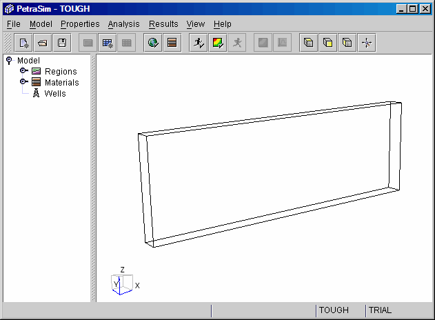
Start PetraSim by selecting Start/Programs/PetraSim. Your display will be a blank window in which we can create the model. In PetraSim, we first define the boundary of the model. Select the Define Boundary tool (or Model/Define Boundary…and create the model boundary with Xmin = 0.0, Xmax = 18.6, Ymin = 0.0, Ymax = 1.0, Zmin = 0.0, and Zmax = 6.0, as shown below.

After selecting OK, the basic model will be created. Click on the model and spin it so that it is displayed as shown below. Hold Shift key and drag to pan; hold Alt key and drag to zoom.
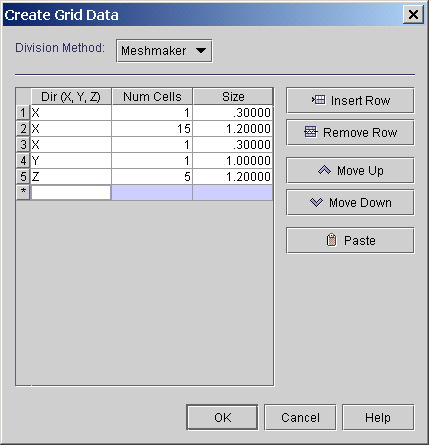
We create the grid on the model by selecting the Create Grid tool (or Model/Create Grid…. Because this example mesh has some small elements and some larger elements, it is easiest to use the Meshmaker type of input, in which the user gives a direction, then number of cells in that direction, and the size of each cell. In PetraSim, the cell definition starts at the minimum coordinate dimension. Select the Meshmaker option and then specify the cells as shown below.
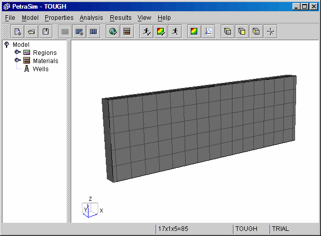
After grid creation, the model is shown below.
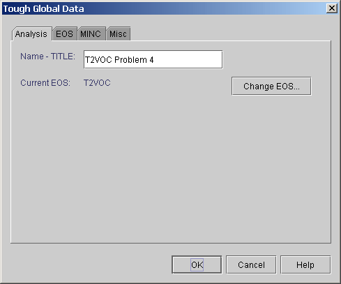
Global properties are those properties that apply to the entire model. Select the Global Properties tool (or Properties/Global Properties…to display a tabbed dialog with Analysis, EOS, MINC, and Misc tabs. First select the Analysis tab and change the Name of the analysis to "T2VOC Problem 4".
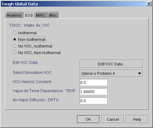
The EOS (Equation of State) tab displays options for T2VOC. In this analysis, we will perform an isothermal (no heat flow) analysis, so select the Isothermal option.
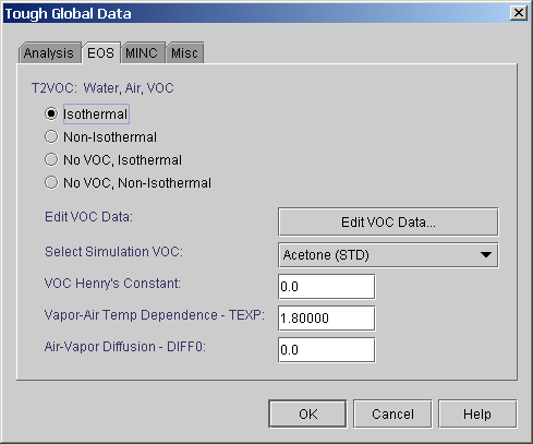
The EOS tab also is where we specify the VOC constants. PetraSim provides a library of standard properties that correspond to the data supplied with the T2VOC distribution. In addition, the user can create their own data sets or modify the existing ones. For this example, we will create a new VOC property set, based on the standard Xylene-o data. Select the Edit VOC Data... button and the Edit VOC Data dialog will be displayed.
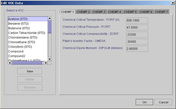
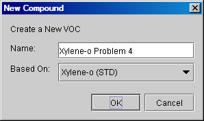
Select the New button to display the New Compound dialog. In this dialog, give the name as "o-Xylene Problem 4" and have the new data set be based on Xylene-o (STD).
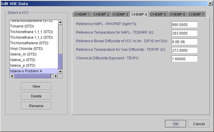
Select OK to create the new data set. The Edit VOC Data dialog will now have the new VOC we just created. There are only a few entries that need to be changed. Select the CHEMP.4 tab and change the Reference Binary Diffusivity to 8.0E-6 m^2/s, the Reference Temperature for Gas Diffusivity to 273 K, and the Chemical Diffusivity Exponent to 1.6.
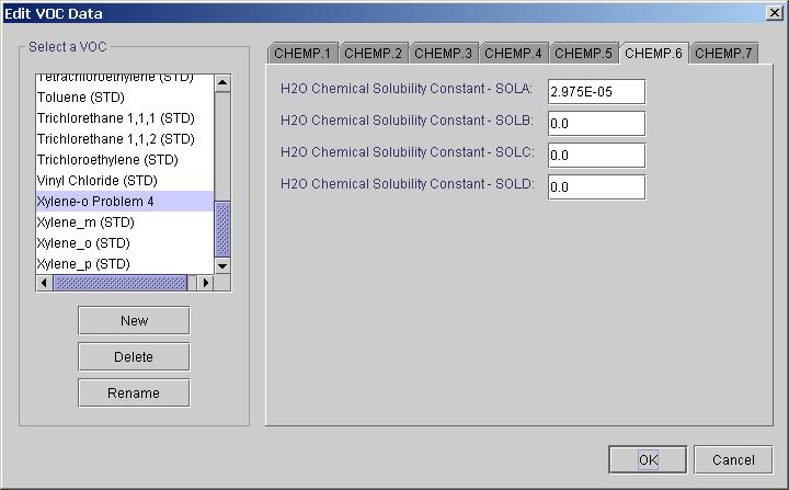
Next, select the CHEMP.6 tab and change the H2O Chemical Solubility Constant - SOLA to 2.975E-5.
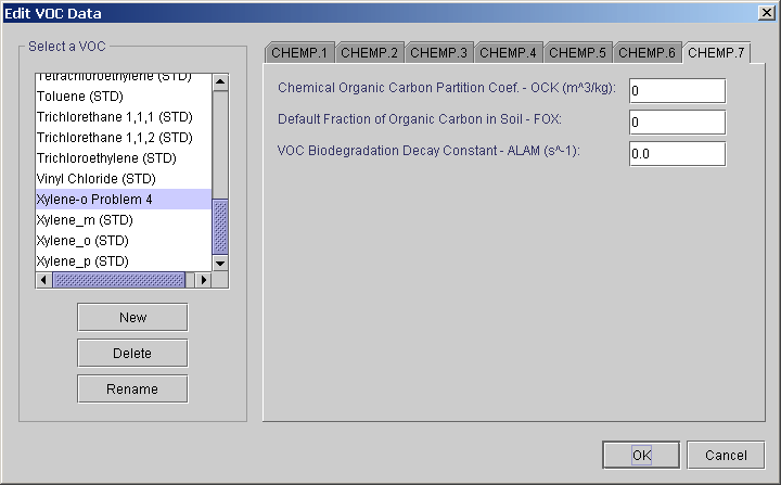
Finally, select the CHEMP.7 tab and set all constants to 0.0.
Select OK to close the Edit VOC Data dialog and select OK again to close the TOUGH Global Data dialog and return to the main window.
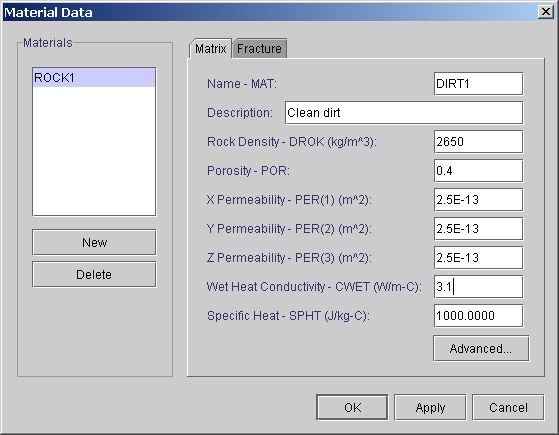
To specify the material properties, select the Material Properties tool (or Properties/Materials... menu) as shown below. Change the material name to DIRT1, the rock density to 2650 kg/m^3, the porosity to 0.4, the permeabilities to 2.5E-13 m^2, the wet heat conductivity to 3.1, and the specific heat to 1000 J/kg-C.
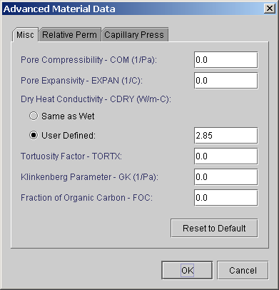
Select the Advanced button to set other options. We will first set the Dry Heat Conductivity to 2.85.
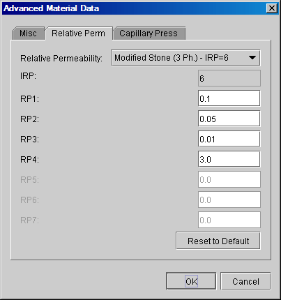
Next, select the Relative Perm tab. This example uses the Modified Stone three phase model for the relative permeability function. Input the constants as 0.1, 0.05, 0.01, and 3.0. To view a plot of this relative permeability, please go to the Tools section of Help/Getting Started on the web and download the relative permeability spreadsheet.
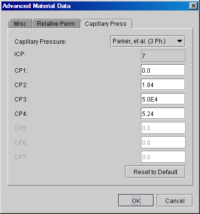
To define the capillary pressure function select the Capillary Press tab and select the Parker model. Input the constants as 0.0, 1.84, 5.0E4, and 5.24.
Select OK to close the Advanced Material Data dialog and the OK to save material data.
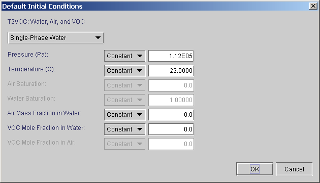
To specify the default initial conditions, select Properties/Initial Conditions…. The default initial conditions represent water at a pressure of 1.12E5 Pa and temperature of 22 C. The air and VOC mass fractions are 0.0.
Select OK to close the Default Initial Conditions dialog.
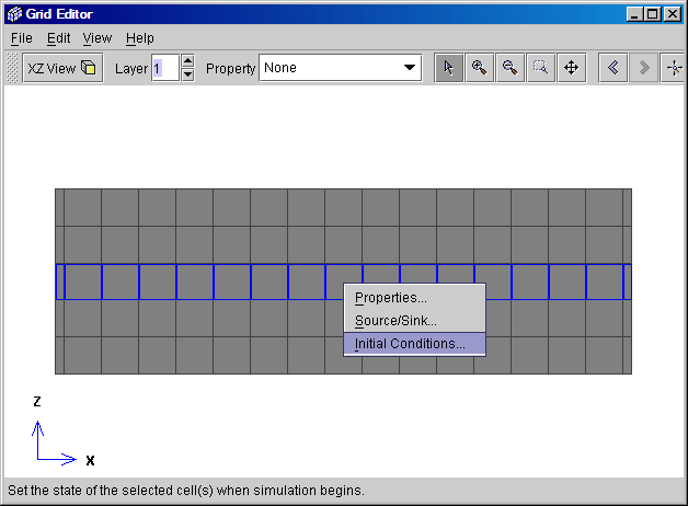
In this problem we modify specific initial conditions to approximate a water table. To do this, select the Edit Grid tool (or Model/Edit Grid menu) and go the the XZ view. Using a click and drag with the mouse, select the upper two rows of cells and then right click on the selected cells.
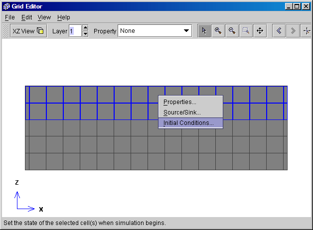
Select Initial Conditions... on the pop-up menu. For all these cells, we will specify a Two Phase Water/Air initial condition with pressure of 1.01E5 Pa, a temperature of 22 C, and a water saturation of 0.1.
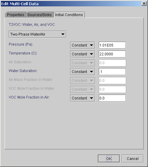
Select OK to close the dialog.
In a similar manner, we will specify the water table in the third row of cells.
For these cells, we will specify a two phase condition with a pressure of 1.01E5 Pa, a temperature of 22 C, and a water saturation of 0.95.
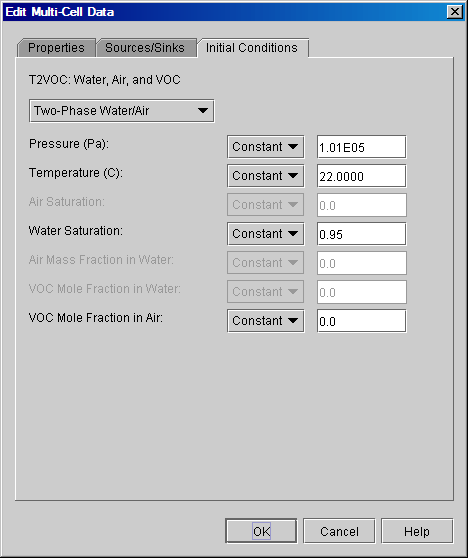
Select OK to close the dialog.
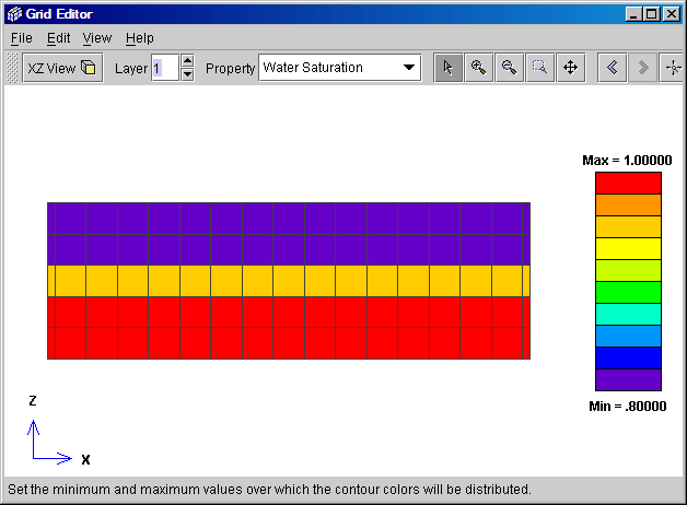
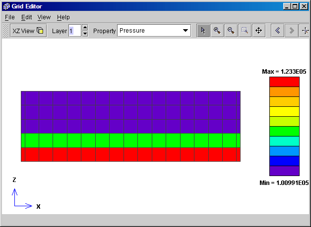
We can display the water saturation by selecting it as the Property to display. In this display, we also selected View/Contour Range and set the minimum value to 0.8. Please be sure to also uncheck the Default Bounds check box to turn off the automatic range calculation. We select the range from 0.8 to 1.0 because PetraSim uses only 10 contour colors, so the default min and max range results in both a saturation of 0.95 and 1.0 being in the same color band.
Close the Grid Editor window.
We next specify the information that will control the solution by selecting the Solution Controls tool (or Analysis/Solution Controls… menu). The Times tab allows us to specify parameters associated with the start and ending of the analysis and the time steps used for the calculation. In this case, we will start at 0 sec, but not specify an end time. Instead, we limit the maximum number of time steps to 20. We also specify the first time step size as 100 sec.

The default values for all other options are satisfactory, so select OK to save the changes.
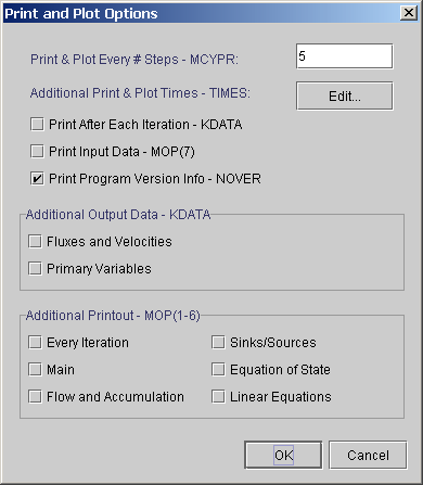
We next specify the information that will control the output by selecting Analysis/Output Controls…. Plot data is read from the TOUGH2 output file. We will output data every 5 time steps.
Select OK to save the changes.
We have now completed the input necessary to write the T2VOC input file. Save the PetraSim file by selecting File/Save… and save the file with the name t2voc_prob4_part1.sim (the *.sim extension will be added automatically if you do not give it).
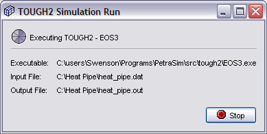
Now run the analysis by selecting Analysis/Run TOUGH2... . During execution the following dialog will be displayed.
At the end of the analysis, the dialog will change to indicate that the analysis is finished.
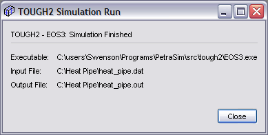
Select the Close button.
If you just want to look at the results without running the analysis, please download the output files that we have already calculated. Links to these files are given at the beginning of this example.
To view the progress of an analysis, the user can open the output file in an editor. As each new time step is written, the user can update the view. Similarly, in PetraSim, the user can make a 3D display of the available results in the output file. Close and reopen the 3D results window to refresh for new data.
After the analysis is complete, select the 3D Results tool (or Results/3D Results... menu). This will display a 3D results window. Since our model is thin, the default iso-surface plots are not too useful. To add a plane on which the results are contoured, select Slice Planes... and the define a plane normal to the Y axis at a position of 0.5 m.
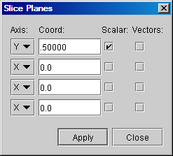
Close the Slice Planes dialog.
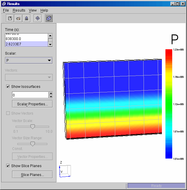
Select pressure as the plot variable, set the number of isosurfaces to 0 and select the last time.
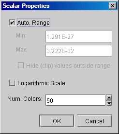
Double click on the Scalar Legend (or select Results/Scalar Properties menu) and set the Number of Colors to 50. This gives a smooth gradation of color contours.
Zoom and pan (Shift key and drag to pan; Alt key and drag to zoom) to create a plot as shown below. The pressure gradient increases in the water saturated zone.
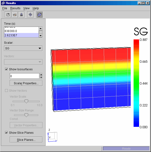
The gas (air) saturation is shown below. Air fills most of the upper portion of the model.
Close the results window.
If not already open, start PetraSim and open the t2voc_prob4_part1 model. We will now save this model to a new directory. Select File/Save As and save the model as t2voc_prob4_part2. Put this file in a new directory that is different than the directory used for the first analysis. This is necessary because TOUGH2 writes output files to its current directory and we want to avoid overwriting that old analysis.
We will first read the results saved in the previous analysis as the initial conditions for the new analysis. Select File/Load Initial Conditions and open the SAVE file that is located in the directory in which the previous analysis was run. The SAVE file is automatically written by TOUGH2 at the end of an analysis and defines the state at that time.
To make sure these results have been loaded correctly, select Model/Edit Grid, go to the XZ view, and plot Pressure. You should see the display shown below.
Close the Grid Editor.
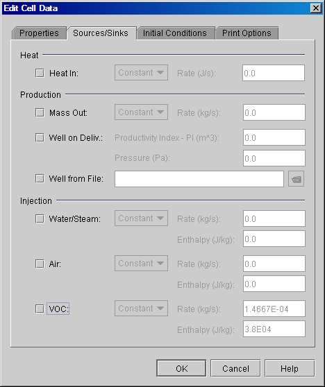
In the next part of the analysis we will define the injection of xylene-o for a period of 4.8E6 sec (55.6 days). The injection rate is 1.4667E-4 kg/s at an enthalpy of 3.8E4 J/kg. The xylene-o is injected into the top center of the model.
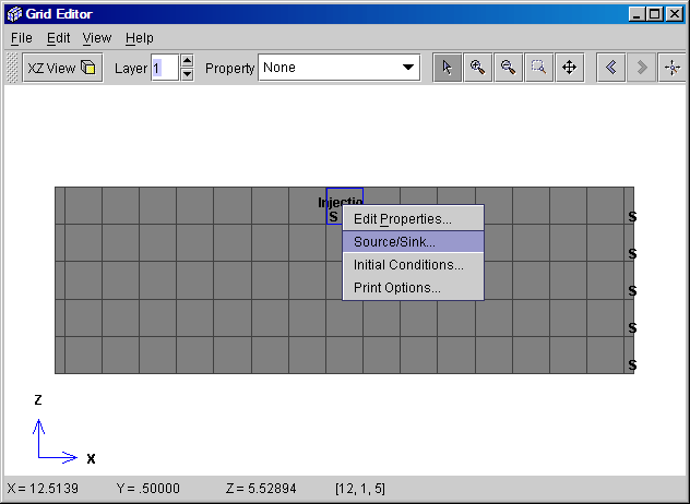
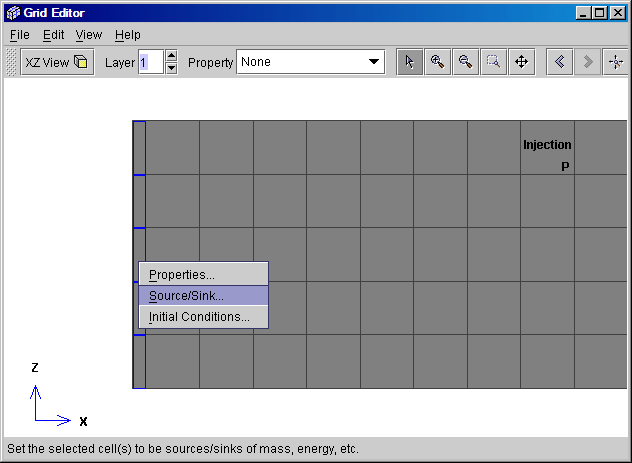
To define this injection, select the Edit Grid tool (or Model/Edit Grid menu) and go to the XZ View. Right click on the top center cell and then select Source/Sink from the pop-up menu.
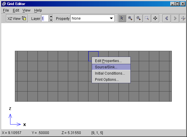
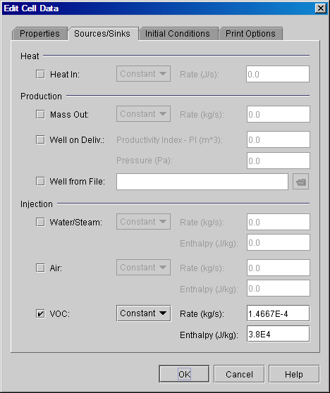
In the Source/Sink tab, select VOC Injection and give the flow rate as 1.4667E-4 kg/s and the enthalpy as 3.8E4.
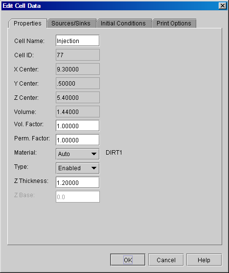
For this cell, we will also demonstrate how to name and plot the cell history. Select the Properties tab and give the Cell Name as "Injection".
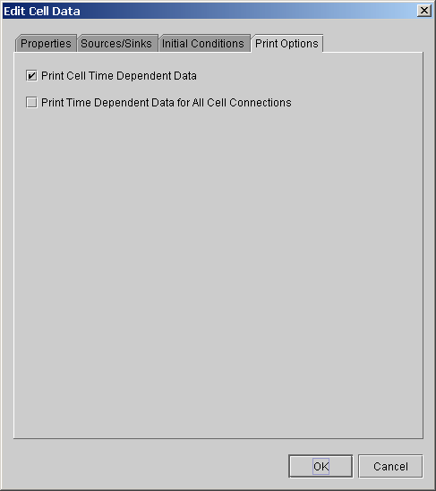
Next, select the Print Options tab and select the Print Cell Time Dependent Data checkbox. This will output data into the FOFT file. Also, since this cell is a source/sink, the GOFT file data will be written by default.
Select OK to close the dialog.
We will also define a deliverability condition on the right of the model. This condition defines a pressure and a productivity index (resistance) for flow to that pressure. In this analysis, the deliverability boundary condition represents an outlet for the flow as the xylene-o is injected. To define the boundary condition, use a click and drag selection with the mouse (or hold down the Cntrl key and click on individual cells) to select the five cells on the right of the model. After these are selected, right click on the cells to display the pop-up menu.
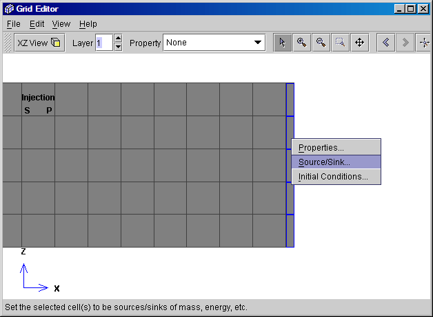
Select Source/Sink in the pop-up menu and select Well on Deliv. for the Production type. Specify the productivity index as 2E-12 and the pressure as 1.232E5 Pa. Note: Review the 3D T2VOC example to see a boundary definition that uses a different pressure for each layer, more closely matching the initial state.
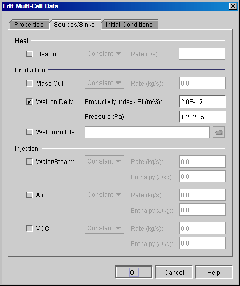
Select OK to close the dialog. Close the Grid Editor window.
For part 2 of the analysis we will start at 0.0 and end at 4.8E6 sec (55.6 days). Specify the time as 4.8E6 sec, the maximum number of time steps as 500, and the initial time step as 100 sec.

Select OK to close the dialog.
We have now completed the input necessary to write the T2VOC input file. Save the PetraSim file by selecting File/Save….
As before, execute the analysis by selecting the Run tool (or Analysis/Run TOUGH2... menu). To start the analysis, select the Start button in the Run Tough dialog. At the end of the analysis, the dialog will change to indicate that the analysis is finished. Close the execution dialog.
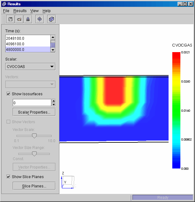
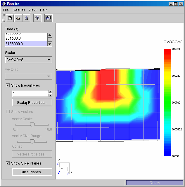
After the analysis is complete, select Results/3D Contours... . As before, define a Slice Plane, then select CVOCGAS as the variable to plot, select the last time, and set the number of colors to 50. The resulting contour is shown below. Note that because the mesh is very coarse, there is some interpolation bias introduced into the plot.
Select the Cell History Plots tool (or Results/Cell History Plots menu) to make a time history plot of the cell data. All data stored in the TOUGH2 FOFT file is available for plotting. Unfortunately, for T2VOC analysis, the output data is rather limited. A plot of Gas Saturation is shown below in the injection element.

Close all results windows.
If not already open, start PetraSim and open the t2voc_prob4_part2 model. We will now save this model to a new directory. Select File/Save As and save the model as t2voc_prob4_part3. Put this file in a new directory that is different than the directory used for the first analysis. This is necessary because TOUGH2 writes output files to its current directory and we want to avoid overwriting that old analysis.
We will first read the results saved in the previous analysis as the initial conditions for the new analysis. Select File/Load Initial Conditions and open the SAVE file that is located in the directory in which the part 2 analysis was run.
To make sure these results have been loaded correctly, select the Edit Grid tool (or Model/Edit Grid menu) go to the XZ view, and plot Pressure.

Close the Grid Editor.
In part 2 of the analysis, xylene-o was injected. In this part of the analysis, we will stop the injection and let the xylene-o diffuse for 3.156E8 sec (10 years). To remove the injection from the model, select Model/Edit Grid and go to the XZ View. Right click on the top center cell and then select Source/Sink from the pop-up menu.
In this dialog, unselect the check on the VOC Injection.
Close the Edit Cell Data dialog and the Grid Editor window.
For part 3 of the analysis we will start at 0.0 and end at 3.156E8 sec (10 years).

Select OK to close the dialog.
We have now completed the input necessary to write the T2VOC input file. Save the PetraSim file by selecting File/Save….
As before, execute the analysis by selecting Analysis/Run TOUGH2... . To start the analysis, select the Start button in the Run Tough dialog. At the end of the analysis, the dialog will change to indicate that the analysis is finished. Close the execution dialog.
After the analysis is complete, select Results/3D Contours... and plot CVOCGAS at the last time, as shown below.
Close the results window.
If not already open, start PetraSim and open the t2voc_prob4_part3 model. We will now save this model to a new directory. Select File/Save As and save the model as t2voc_prob4_part4. Put this file in a new directory that is different than the directory used for the first analysis.
We will first read the results saved in the previous analysis as the initial conditions for the new analysis. Select File/Load Initial Conditions and open the SAVE file that is located in the directory in which the part 3 analysis was run.
To make sure these results have been loaded correctly, select Model/Edit Grid, go to the XZ view, and plot Pressure. Your display should appear as below.

Close the Grid Editor window.
In this part of the analysis, we will inject steam into the model. To enable a non-isothermal analysis, select Properties/Global Properties and select the Non-Isothermal option.
Select OK to close the dialog.
In this part of the analysis, we will inject steam on the left side of the model. Open the Grid Editor and go to the XZ View. Use click and drag to select the five cells on the left of the model, then right click on these cells to display the pop-up menu.
Select Source/Sink and then Water/Steam as Injection. The injection rate is 1.48E-4 kg/s for each cell and the enthalpy is 2.676E6 J/kg.
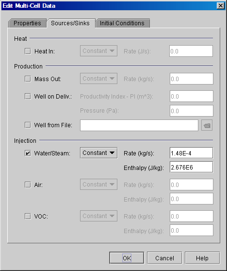
Select OK to close the dialog and then close the Grid Editor window.
For part 2 of the analysis we will start at 0.0 and end at 1.48E7 sec (171 days).
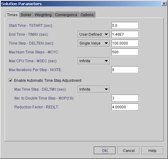
Select OK to close the dialog.
We have now completed the input necessary to write the T2VOC input file. First save the PetraSim file by selecting File/Save….
As before, execute the analysis by selecting Analysis/Run TOUGH2... . To start the analysis, select the Start button in the Run Tough dialog. At the end of the analysis, the dialog will change to indicate that the analysis is finished. Close the execution dialog.
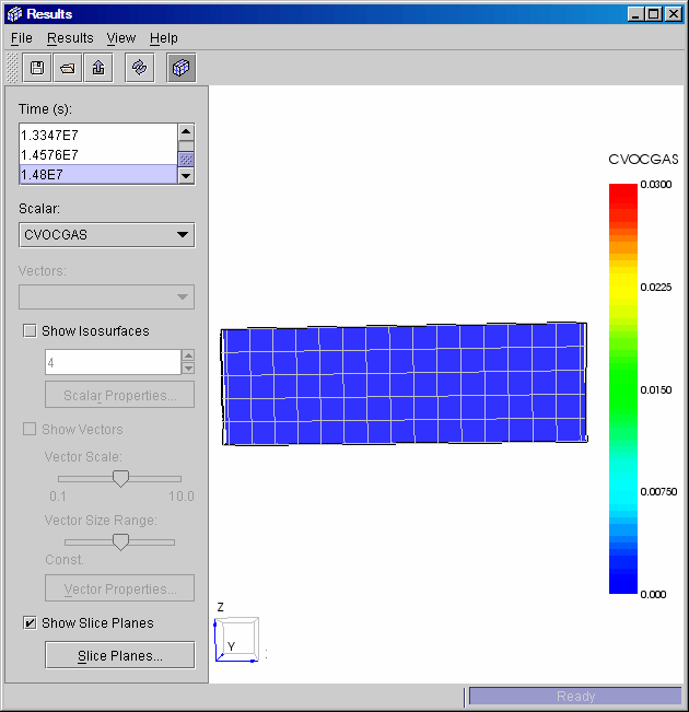
After the analysis is complete, select Results/3D Contours... . Again, define a Slice Plane and select CVOCGAS as the plot variable. We want to set the contour ranges so that they are the same for all plots. To do this, double click on the legend (or Results/Scalar Properties... menu) and then turn off the Auto Range option, set the Min to 0, the Max to 0.03, and set the Number of Colors to 50..
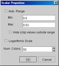
Select OK to close the dialog.
Next, select the plot at time near 4.32E6 sec (50 days). As can be seen, the sweep is starting to remove the NAPL.
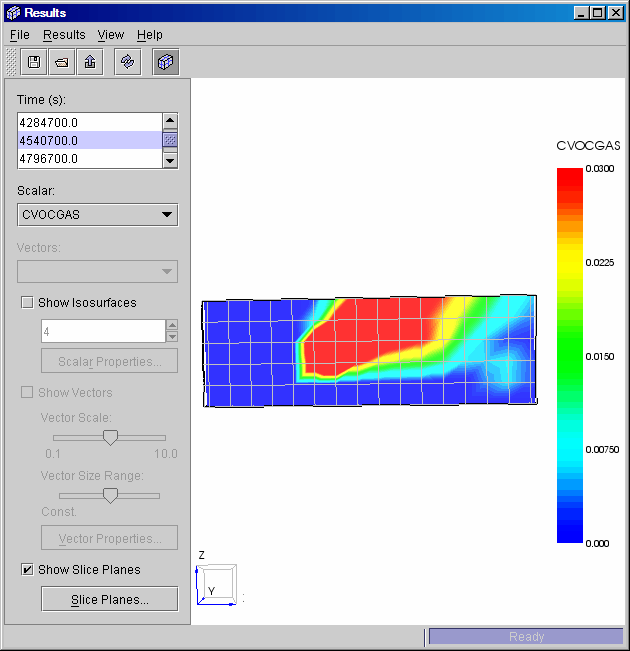
A plot of at the last time shows the NAPL has been removed.
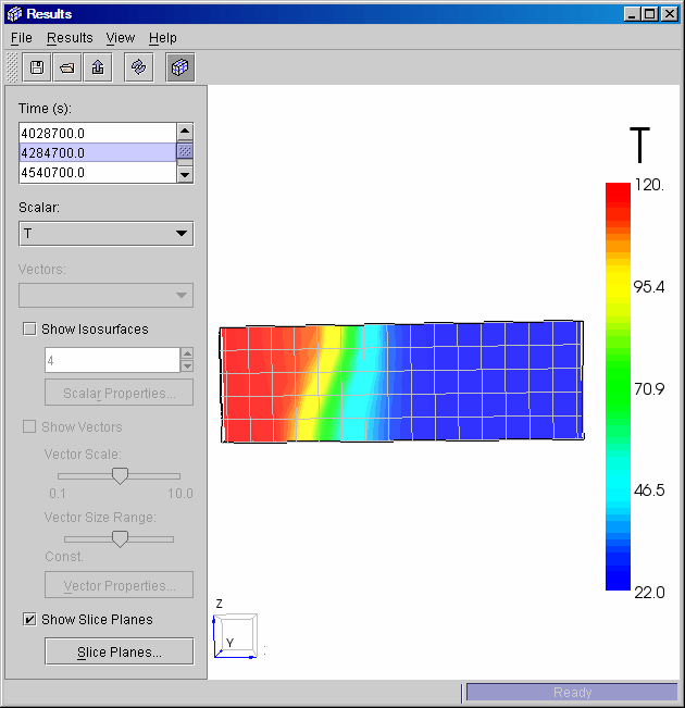
The temperature contours at approximately 50 days are shown below. The heating due to steam injection can clearly been seen.
At the end time, essentially all the NAPL has been removed.